Simple River Network (SRN)¶

Overview¶

The Simple River Network, or SRN, is a graphical, pseudo-physical diagnostic tool used to visualize watershed models. Utilizing NetworkX’s nodal network structure, SRNs represent each river segment, or seg, as a singular SegNode and connects them according to the watershed’s topology. Each SRN is color-codable to assigned data values, such as percent bias, so you can visualize where issues may appear in the watershed during bmorph bias correction to more easily understand spatial patterns of bias correction in the network.

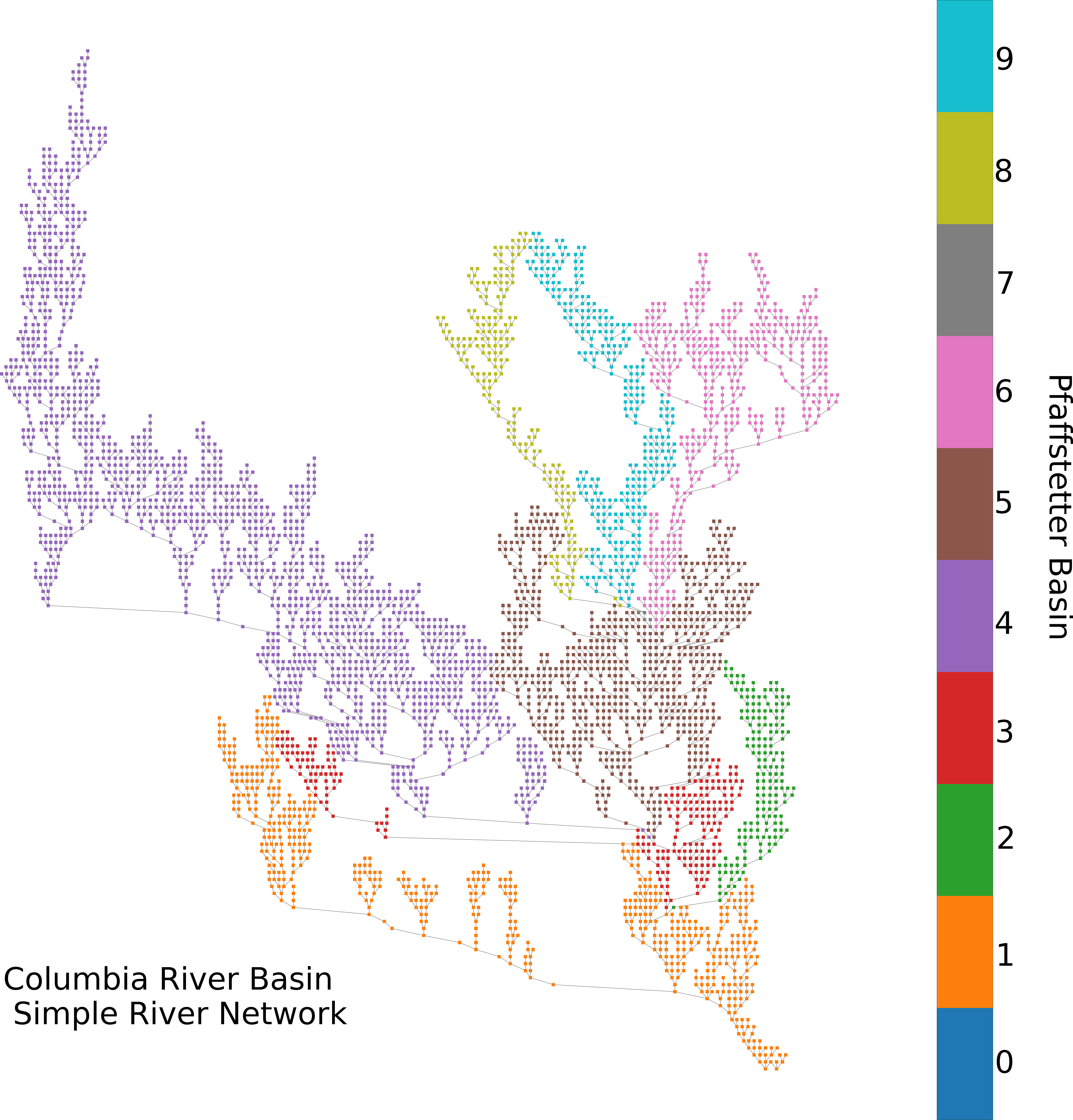
Nodal network of the Columbia River Basin showing river segment connections and color-coded by Pfaffsetter basin.

SRN SegNode’s contain identifying information that allow the network to be partitioned according to Pfaffstetter Codes (Verdin & Verdin 1999, Arge et. al. 2006). Pfaffstetter enconding not only allows the networks to be partitioned, but also to be “rolled up”, effectively reducing the granularity of the network to simplify large watersheds. Data can also be subsetted and split into new SRN’s for simple manipulation.

SRN does not aim to supplant geographically accurate drawings of watershed networks. Instead it aims to provide a quicker, intermediate tool that allows for easy identification of spatial patterns within the network without having to configure spatial data.

Construction¶

from bmorph.evaluation import simple_river_network as srn

srn_basin = srn.SimpleRiverNetwork(
    topo=basin_topo, pfaf_seed='', outlet_index=0, max_level_pfaf=42)

All we need to setup the SRN is the topology of the basin, basin_topo, as an xarray.Dataset. If you wish to include the Pfaffstetter digits of the larger watershed that contains the basin, you can do so with pfaf_seed. While the constructor will assume that the outlet of the basin is the first index of the topology file provided, you can specify a different index to build the SRN off of with outlet_index. Lastly, because the SRN is constructed recursively, a maximum number of Pfaffstetter digits is specifiable in max_level_pfaf, which defaults as 42. Note that the larger the basin SRN, the longer construction may take.

Plotting on the SRN¶

Plotting the SRN is fully describe in bmorph.evaluation.simple_river_network.SimpleRiverNetwork.draw_network, so let’s cover some of the basics.

Plotting data on the SRN is done through draw_network’s color_measure that requires a pandas.Series with and index that contains the indices of basin_topo and corresponding values to be plotted on a linear colorbar. Several functions automate this process for highlighting different sections of the SRN, such as bmorph.evaluation.simple_river_network.SimpleRiverNetwork.generate_mainstream_map to plot the mainstream, bmorph.evaluation.simple_river_network.SimpleRiverNetwork.generate_pfaf_color_map to color code Pfaffstetter basins, and bmorph.evaluation.simple_river_network.SimpleRiverNetwork.generate_node_highlight_map to highlight specific river segments within the drawing.

mainstream_map = srn_basin.generate_mainstream_map()

fig, ax = plt.subplots(figsize=(30,40))
srn_yak.draw_network(color_measure=mainstream_map, cmap=mpl.cm.get_cmap('cividis'), ax=ax)
ax.invert_xaxis() # inverting the axis can be applied to increase resemblance with real watershed

For an example of how to construct your own color_measure, we can look at how the tutorial plots percent difference across the SRN:

scbc_c = conditioned_seg_totals['IRFroutedRunoff']
raw = yakima_met_seg['IRFroutedRunoff']
p_diff = ((scbc_c-raw)/raw).mean(dim='time')*100

percent_diff = pd.Series(data=p_diff.to_pandas().values,index=mainstream_map.index)

fig, ax = plt.subplots(figsize=(30,40))
srn_yak.draw_network(color_measure=percent_diff, cmap=mpl.cm.get_cmap('coolwarm_r'),
                 with_cbar=True, cbar_labelsize=40, ax=ax, cbar_title='Percent Difference (%)')

The SRN is compatible with subplotting, but may require a large subplot space to spread out.

Citations¶

Arge, L., Danner, A., Haverkort, H., & Zeh, N. (2006). I/O-Efficient Hierarchial Watershed Decomposition og Grid Terrain Models. In A. Riedl, W. Kainz, G.A. Elmes (Eds.), Progress in Spatial Data Handling (pp. 825-844). Springer, Berlin, Heidelberg. https://doi.org/10.1007/3-540-35589-8_51

Verdin, K.L., & Verdin, J. P. (1999). A topological system for delineation and codification of the Earth’s river basins. Elsevier Journal of Hydrology, 218, 1-12.